Option Strategies Performance

The whole methodology of the Fair Value and market mispricing for a single option contract can also be applied to the options multi-leg combinations (strategies).

This section of the Working Area presents the various performance metrics of such options combinations: Fair Value, Market Price, Expected Profit/Loss, risk-adjusted returns, etc., calculated for the selected Filter Bin.

Control Panel

The area for all presets and parameters:

1.Strategy selector

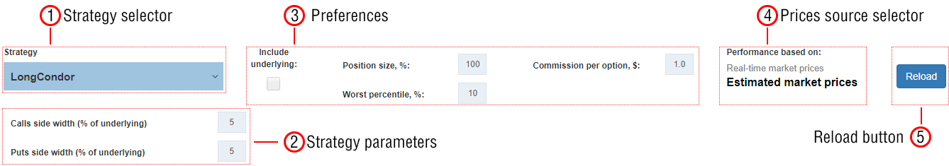
Select a strategy to evaluate from the dropdown list:

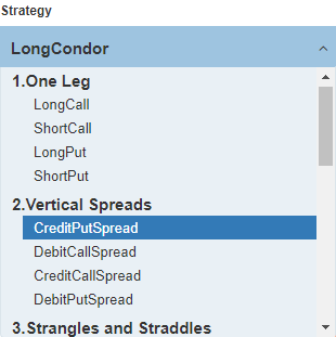
The complete list of strategies is here. 

2.Strategy parameters

For several multi-leg strategies, it is necessary to set some additional parameters to limit the number of possible legs combination:

• Condors: call and put wings size,
• Butterflies:  moneyness of the central strike
• Ratio and Back Spreads: ratio of OTM to ITM legs

For the other strategies, no such parameters are needed because all possible legs combinations for them can be presented in at least a 2D format (matrix or table, see below).

3.Preferences

• Include underlying – if checked, the long underlying security will be added to the strategy, transforming the strategy type (Short Call to Covered Call, Bear Risk Reversal to Collar, etc.)
• Position size – the ratio that translates the basic return metrics (see below) into the Return on Portfolio (RoP)
• Worst percentile – the risk tail parameter of the probability level for two metrics: RoP percentile and average RoP below this level
• Commission per option – total trading commission per one option contract, in $

4. Prices sources selector

It is possible to calculate the performance against either historical Estimated Prices or real-time market prices. By default, all metrics are calculated for the historical prices if they are available for the security. The real-time option is not available until the respective prices have been loaded.

Some metrics, which require a historical data series and the respective probability distribution (tail risk parameters, standard deviation, Sharpe/Sortino ratios, etc.), are not available for the performance calculated with the real-time prices.

5. Reload button

Recalculates all metrics according to the preferences and parameters set in this panel.

Performance metrics

The main calculation workflow for the performance metrics:

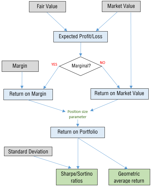
The key steps:

Step 1. Fair Value, Market Value, Expected Profit/Loss

Initially, the Fair and Market Values are calculated for each leg of the combination and summed up to get these values for the whole strategy (see the methodology article). 

Expected Profit/Loss is just a difference between the Fair Value and the Market Value (either historical or real time) for long strategies and vice versa for the short ones. All three metrics are calculated as a percentage of the underlying price with the same logic as with the single option contract.

Note that this logic is feasible only if all the option legs have the same expiration date (Fair and Market values must be additive), that is why the calendar/diagonal strategies are not applicable here.

Step 2. Basic return metrics

Depending on the margin requirements for the strategy (either a margin is required or not), the basis for the returns is the following:

• Margin – for marginal positions – the Return on Margin (RoM) calculation
• Market Value – for non-marginal positions – the Return on Market Value (RoMV) calculation

For the Marginal strategies, RoMV is also calculated and displayed but just as a reference without further usage in the calculation workflow.

Two types of a Margin are used:

• Initial margin – for the strategies with open risk (i.e., having the “naked” legs). That margin will change with the underlying price movement, and all the RoM metrics will also change.
• Maximum loss – for the strategies with defined risk (i.e., spreads, condors, etc.). That margin does not change in the lifetime of the position.

The margin calculation complies with the Strategy-based margining rules of CBOE for cash accounts (the most conservative approach).

Adding an underlying security to the position (checkbox Include underlying) changes this returns basis from Margin to Market Value. So that the Short Call becomes Covered Call, the Bear Risk Reversal becomes Collar, etc. All that strategies with underlying security are considered as non-marginal.

Step 3. Return on Portfolio

The basic returns (either RoM or RoMV) are transformed into the Return on Portfolio (RoP) metrics with the Position Size parameter, which is manually set in the control panel of this section.

For instance, if we set the Position Size to 50% for some marginal strategy, our Portfolio will be margined by 50%. For a non-marginal position, we will buy options with the total market value of 50% of the total Portfolio. In this example, our Return on Portfolio will be half of the RoM and RoMV, respectively (with the comparable risk reduction, obviously).

Step 4. Risk-Adjusted Return on Portfolio

If the performance metrics are calculated on the basis of historical Estimated Prices, we have the whole series of profits/losses on each date in history. That allows us to calculate the various risk metrics and the respective risk-adjusted returns. The most common metrics are the Standard Deviation of returns and the Sharpe ratio, which are calculated for the Return on Portfolio.

Besides that, some other risk metrics are calculated:

• Standard Deviation down and Sortino ratio,
• Probability of loss,
• Median and Worst RoP,
• Worst RoP percentile (the parameter set in the Control Panel) and the average RoP below that value

Geometric Average Return on Portfolio employs the capitalization of profit/loss with the following formula:

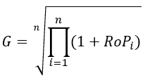
This is an average Return on Portfolio with the compounding of each historical RoP. It contrasts with the average Return on Portfolio calculated as an arithmetical average to get the mathematically expected return.

Position sizing

This is the optimal ratio of Margin/Market Value to the size of the whole portfolio maximizing the total compounded return. It is calculated with two formulas having slightly different approaches:

• Kelly Criterion – the optimal bet size calculated with the following formula:

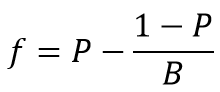
P – the win probability – the ratio of all profitable trades to the total number of trades

B – ratio of amount won on a winning bet to amount lost on a losing bet

This formula can also be presented as a ratio of the expected return (average RoP) to the expected return in case of profit (average positive RoP)

• Optimal Position Size –  the position size level maximizing the geometric return, see above the respective formula.

Both these values serve the same purpose: they find a position size that would maximize the total return.The Kelly criterion, although being well known, considers all losses and wins as being of the same size (it operates average win to average loss ratio, see the formula above). The Optimal Position Size, therefore, is preferable since it directly calculates the position size maximizing the Geometric return.

Here is how usually the Geometric return depends on the position size parameter:

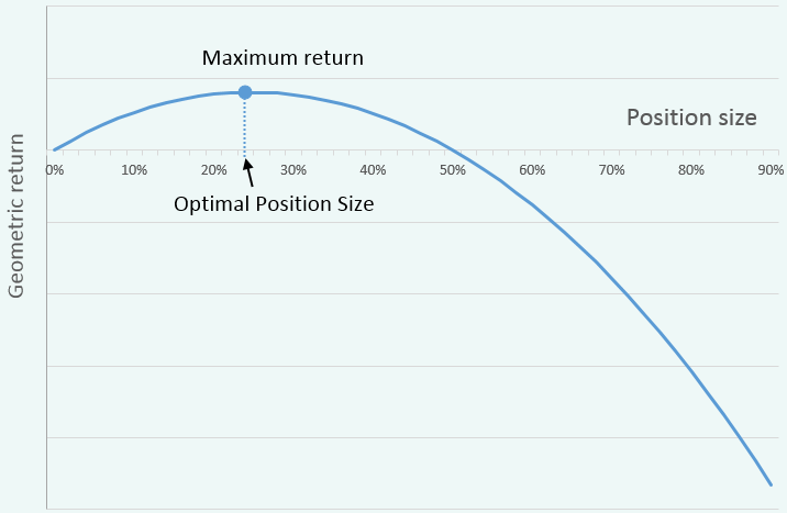
The Optimal Position Size is a point at which the Geometric return is maximized. Notice how it turns negative after some level of position size (around 50%).  It is so-called “overbetting” level when the position size is too big and becomes detrimental to the total portfolio performance (if returns are compounded, of course).

Performance metrics tables and matrices

All performance metrics are presented in two formats depending on the number of the strategy legs:

• One-dimensional table – for one-leg strategies or the strategies with the same strike for all legs (such as Straddle)
• Two-dimensional matrix – for the strategies with two or more legs with different strikes

One-dimensional table

All results are presented in one table: performance metrics – in its rows, moneyness of options – in columns.

Here is an example of the Long Call strategy with 10% Position Sizing:

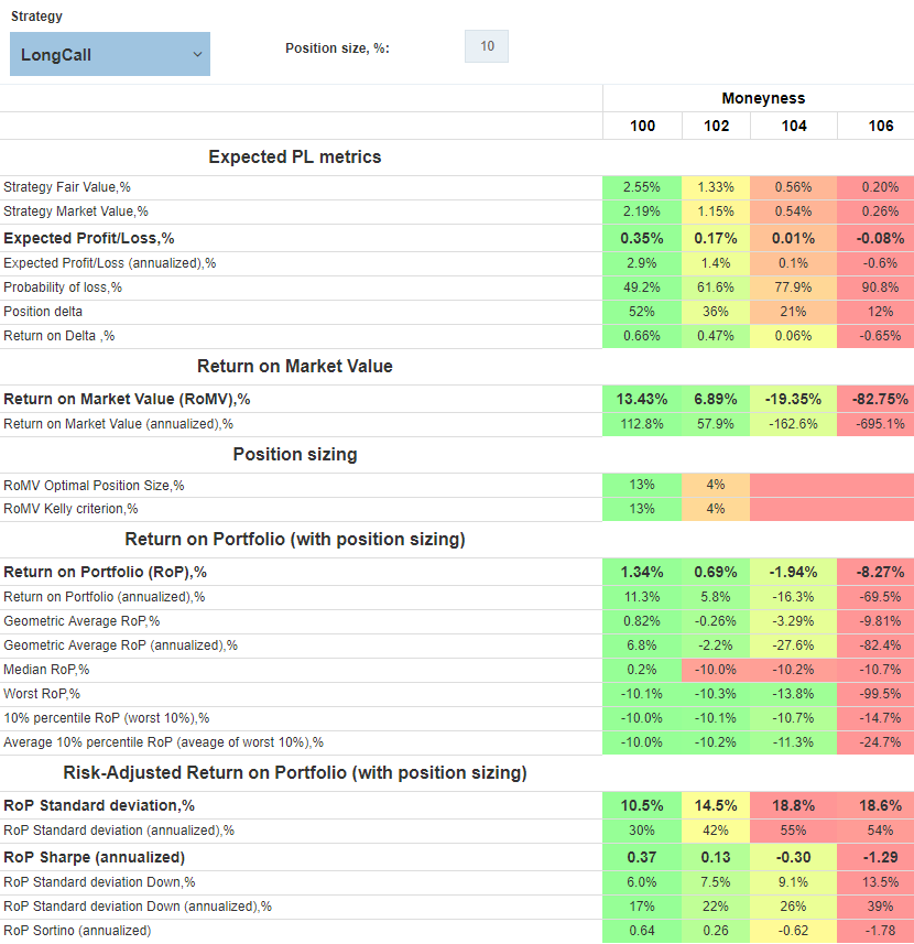
The color gradient from red to green visually highlights the variability of the values of different moneyness (columns).

The Return on Market Value section in this example will be replaced by the Return in Margin for the marginal positions (see the metrics calculation workflow). However, adding an underlying security (checkbox Include underlying) makes them non-marginal and changes their returns basis from Margin to the Market Value.

Two-dimensional matrices

In this format, each metric is presented in one separate matrix with one parameter in rows and another one in columns.

This is an example of the CreditPutSpread strategy with 50% Position size:

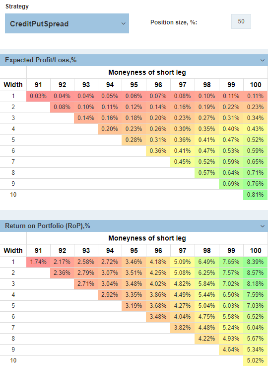
This strategy has two parameters:

• Moneyness of short leg – columns
• Spread width – rows

That matrix presents all possible combinations of Moneyness and Width with the option contracts built according to the Moneyness range and step preference in the main Control Panel. The gradient color highlights the areas with maximum and minimum levels of the selected performance metric.

Depending on the particular strategy, rows and columns can present different parameters. For instance, for Condors, they are the moneyness of short call (columns) and short put (rows) legs.

Strategy Mispricing Chart

The Fair Value of a strategy can be visually compared to its Market Value on a chart similar to the Mispricing Chart for a single contract. It is located:

• For the strategies with one-dimensional tables – directly below the Control Panel (collapsed by default)

• For two-dimensional strategies – by clicking either on a column header of any matrix (iterates all rows on the chart’s horizontal axis) or on a row header (iterates all columns)

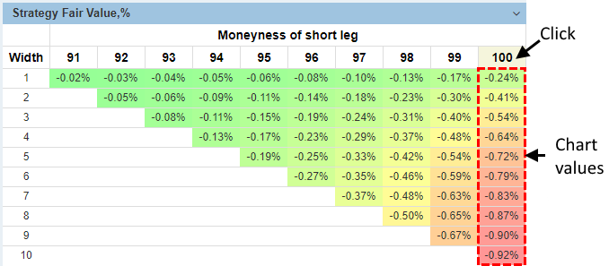
Here is an example of the Credit Put Spread mispricing chart with the short leg moneyness of 100 (appeared after clicking on the column with 100 moneyness):

Negative values indicate that this is a “credit” strategy, and buying it means actually selling a put option with the buying of another one, farther OTM. The total credit is to be accrued to the account.

The Fair Value boxplots are constructed analytically with the same algorithm as for a single contract.

Performance Dashboard

Every strategy with a particular set of parameters can be further “drilled-down” by clicking on any cell within a table or a matrix. All statistics and metrics will appear in the Performance Dashboard window.

Here is an example of the Credit Put Spread with 98 moneyness of the short leg and width of 4 (98-4=94 moneyness of the long leg):

1. Strategy legs

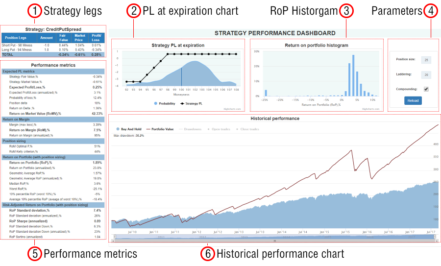
All legs of the strategy are presented in the table format with the following information about each leg:

• Trade direction, option type and moneyness (e.g., Short Put – 98 moneyness)
• Amount of options per one position
• Strategy Fair Value
• Strategy Market Price
• Expected Profit/Loss as a difference between the Fair Value and the Market Price

2.PL at expiration chart

Profit/Loss of the strategy at expiration is presented with the probability density chart demonstrating the probability of expiration at a particular strike (moneyness). The probabilities are calculated on the basis of the actual distribution of the underlying security price in the selected Filter Bin.

Actually, the strategy Expected PL is the sum of the products of these two charts: all possible PLs at expiration weighted by their probabilities. This is the logic of the mathematical expectancy calculation – the same as for the Fair Value but incorporating the Market Price of the strategy.

3. Return on Portfolio Histogram

A histogram chart demonstrating the of Return on Portfolio distribution.

4. Parameters:

• Position size – the same parameter as in the Control Panel transforming the Return on Margin/Market Value into the Return on Portfolio metrics
• Laddering – parameter for the Portfolio Value (Equity line) indicating how many steps should each expiration cycle be divided into, see below – Historical Performance Chart.
• Compounding – whether or not to capitalize all the profit/losses when Portfolio Value (Equity line) is constructed

The Reload button  recalculates all the data in this dashboard according to these parameters

5. Performance metrics

The same metrics as in the main section.

The Return on Portfolio and related metrics can be recalculated with the Position size parameter without closing the Dashboard window.

6.Historical performance chart

This chart contains the Portfolio Value (Equity line) diagram in comparison with the Buy&Hold strategy with the underlying security.

Both lines have a start at the level of 100 and imitate the following trades:

• Buy and Hold series emulated buying the underlying securities on 100% of the portfolio value at the first day and hold this portfolio until the end of the period. Since the underlying security series are dividends/splits adjusted, that line simulates the total return of the underlying security portfolio with dividends reinvestment.
• Portfolio Value series emulates the buying of the option strategy with the following position sizing algorithm:

First, according to the Position size parameter, the total share of the portfolio to be put at risk is determined.

Second, that part of the portfolio is divided into the pieces according to the Laddering parameter. For instance, Laddering 10 means the portfolio at risk is divided into 10 equal parts. Each of these parts considered as a separate trade and is made at the equal time intervals of the length calculated as a division of the days-till-expiration (DTE) of the options to the Laddering parameter.

• Drawdowns (turned off by default)- Portfolio Value drop from the last peak value

For example, if we analyze the strategy with options having 20 days to expiration (DTE) and set the Laddering to 10, Position size to 50%, the system will enter the market with time interval of 20/10=2 days with the trade size of 50/10=5% of the portfolio.

By default, the Laddering is set equal to the DTE of the options (Interval parameter in the main Control Panel). That means the system will enter the market every day with the share of the portfolio calculates as Position Size/DTE.

The Laddering of 1 leads to the sequential trading when each next opening occurs at the expiration of the previous position. In this case, since there is no intermediate mark-to-market repricing, the Portfolio Value line will have “steps” and look like a “ladder.” Here is the Credit Put Spread, 98/94 moneyness, 20 DTE (with drawdowns series turned on):

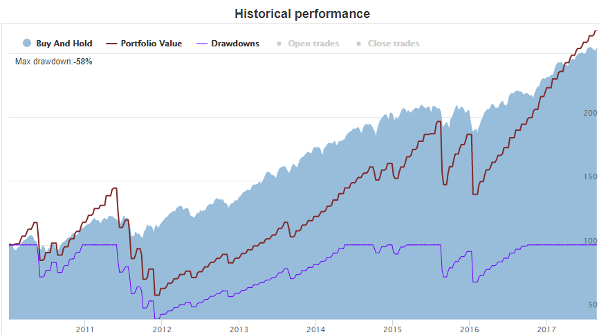
All the trades are made at the historically Estimated market prices and not at the actual historical quotes, which did not exist on each day in history. For more about the rationale and the calculation algorithm, see the respective methodology article.

It is possible to show all the trades on the chart (the respective series are turned off by default): green dots are the opening trades, red dots are the closing ones. Hovering the mouse over these dots pops up all the details:

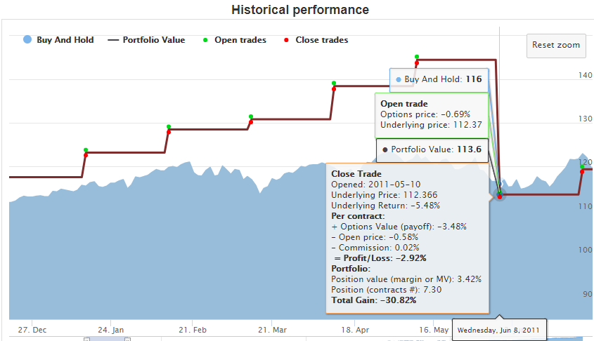
Each closing trade has the detailed breakdown of the Profit/Loss, the size of the position, and the total gain to the portfolio.

Strategy types

The OptionSmile platform calculates the performance for the following strategies:

Strategy	PL profile	Legs	Parameters	Return basis	Long underlying allowed
1.One Leg
ShortPut		Short Put	–	Margin	No
ShortCall		Short Call	–	Margin	Yes
LongPut		Long Put	–	Market Value	Yes
LongCall		Long Call	–	Market Value	No
2.Vertical Spreads
CreditPutSpread		Short ATM Put Long OTM Put	–	Margin	No
DebitPutSpread		Long ATM Put Short OTM Put	–	Market Value	Yes
CreditCallSpread		Short ATM Call Long OTM Call	–	Margin	Yes
DebitCallSpread		Long ATM Call Short OTM Call	–	Market Value	No
3. Strangles and Straddles
ShortStraddle		Short Call Short Put	–	Margin	No
LongStraddle		Short Call Short Put	–	Market Value	No
ShortStrangle		Short Call Short Put	–	Margin	No
LongStrangle		Short Call Short Put	–	Market Value	No
4.Condors and Butterflies
ShortCondor		Short OTM Put Long ATM Put Long ATM Call Short OTM Call	Calls side width Puts side width	Margin	No
LongCondor		Long OTM Put Short ATM Put Short ATM Call Long OTM Call	Calls side width Puts side width	Market Value	No
ShortPutButterfly		1 Long OTM Put 2 Short ATM Put 1 Long ITM Put	Central strike moneyness	Margin	No
LongPutButterfly		1 Short OTM Put 2 Long ATM Puts 1 Short ITM Put	Central strike moneyness	Market Value	No
ShortCallButterfly		1 Long OTM Call 2 Short ATM Calls 1 Long ITM Call	Central strike moneyness	Margin	No
LongCallButterfly		1 Short OTM Call 2 Long ATM Calls 1 Short ITM Call	Central strike moneyness	Market Value	No
5.Ratio Spreads
RatioPutSpread		Long ATM Put (r) Short OTM Put	Ratio of OTM to ATM legs	Margin	No
RatioCallSpread		Long ATM Call (r) Short OTM Call	Ratio of OTM to ATM legs	Margin	No
BackPutSpread		Short ATM Put (r) Long OTM Put	Ratio of OTM to ATM legs	Market Value	No
BackCallSpread		Short ATM Call (r) Long OTM Call	Ratio of OTM to ATM legs	Market Value	No
6. RiskReversals
BullRiskReversal		Short OTM Put Long OTM Call	–	Margin	No
BearRiskReversal		Long OTM Put Short OTM Call	–	Margin	Yes
BullRiskReversalHedged		Long OTM Call Short OTM Put Long farther OTM Put	Hedging leg distance from short leg	Margin	No
BearRiskReversalHedged		Long OTM Put Short OTM Call Long farther OTM Call	Hedging leg distance from short leg	Margin	No
7. Others
CashSecuredPut		Short Put Cash	–	Market Value	No
CoveredPut		Short Put Short underlying	–	Margin	No