OptionSmile is a software platform that calculates the Fair Value of options and estimates the expected profit/loss of an option buying or selling – based on the probabilities derived from historical data of underlying security returns.
Here is the theoretical background.
Fair Value is a central concept. It is a price of a derivative security at which
both buyer and seller have zero expected profit

When a market price exceeds this Fair Value, an option contract is overvalued and a seller has an edge over the buyer. In the opposite case, an option is supposed to be undervalued and a buyer has a positive expected profit.
Expected profit – is a mathematically expected financial result. It is calculated via the
weighting of all possible outcomes by their probabilities
The outcome of a derivative – a payoff – is always known and determined by the contract specification. It is, actually, a value of the derivative at expiration. Here are the payoff diagrams for put and call plain vanilla options:
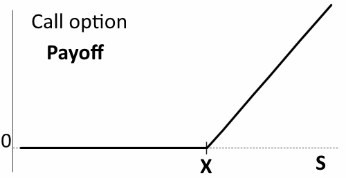
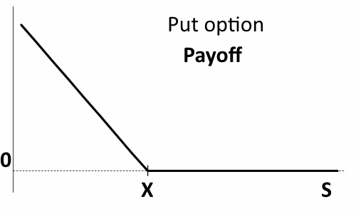
S – price of underlying security
X – strike price of a contract
A payoff diagram is a graphical representation of a Payoff function that returns an option value at the expiration depending on the price of the underlying security (sexp) at that moment. Payoff functions are:
call option: Payoff = Max(0, sexp-X)
put option: Payoff = Max(0, X-sexp)
The remaining and unknown part of the Fair Value are the probabilities of the underlying price to finish at some point – at the option expiration.
Probability density function (probability distribution) returns the probability (P) of some event:
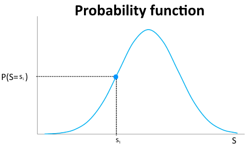
P(S=s1) is a probability of S taking the s1 value. In our case, it is a probability of the underlying security reaching some price s1 at the expiration of an option contract.
Finally, to get a Fair Value of an option we have to take its all possible payoffs (payoff function) and weight them with their probabilities (probability function):
Fair Value = Σ payoff*probability
Here is an example for a put option:
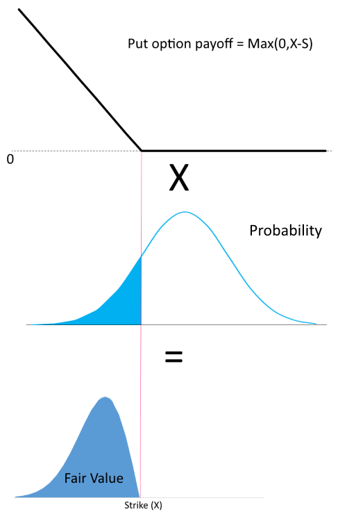
The Fair Value is equal to the shaded area on the lower diagram.
Mathematically speaking, it is calculated by the following integral (click to expand):
Fair Value = 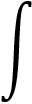 Ps*Vs*ds
Ps – probability of underlying price to reach s at expiration (probability function)
Vs – value of an option in case of underlying price equals s at expiration (payoff function)
The payoff event is expected to occur at some future point. Therefore, the final step is to calculate the present value of the Fair Value to make it comparable to the current market price. That is done with multiplication by discounting factor e-rt, where r – risk-free rate, t – time till expiration.
All above formulas are applicable for all types of derivative securities: futures, options, swaps, warrants, etc. The OptionSmile is focused on the plain vanilla European-style options. That makes the calculation simpler thanks to the payoff function being zero in the out-of-the-money(OTM) area (when price>strike for puts and price<strike for calls).
Actually, it does not matter what the probabilities are in the area when the payoff is zero. Everything multiplied by zero is also equal to zero.
For a put option:
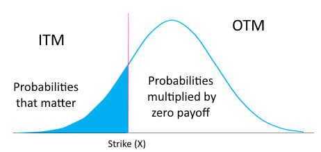
Therefore, we can completely ignore the probabilities in the out-of-the-money zone and simplify the Fair Value Formula:
Fair Value = Pitm * EVitm * e-rt
Pitm – probability of the in-the-money expiration
EVitm – expected value (payoff) of an option in case of ITM expiration (conditional expectation)
e-rt – discount factor
Mathematically speaking, the Fair Value of an options contract is (click to expand):
call option: P(S>X) * E[ S-X | S>X] * e-rt
put option: P(S<X) * E[ X-S | S<X] * e-rt
In other words, it does not matter what goes on in the area where our contract is to expire worthless – in the OTM zone. The only area that matters is ITM.
That formula is similar to the approach used in the insurance industry. The fair insurance premium is equal to the probability of an insured event (claim arrival) multiplied by the expected claim amount (claim severity). In the case you have not had a car accident and have not made a claim to your insurance company, it does not matter whether you have several times been very close to a car crash. It has not actually happened, and the insurance company is not aware of it. Based on the historical data of accidents and some of your personal characteristics — driving experience, age, claims history — they build their actuarial models predicting the probability of a claim and its value (loss for them). Real actuarial models, of course, are much more sophisticated, but the general concept is the same as proposed in the OptionSmile platform.
Another interesting outcome from the Fair Value formula is that a historical or expected volatility of an underlying security, measured by the standard deviation, does not directly influence the Fair Value of options and, hence, the expected profit/loss of options trading. That is especially pronounced for the contracts with ITM/OTM strikes: average deviation from the mean does not always reflect the real probabilities in the particular tail.
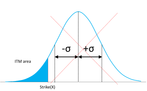
That fluctuation around the mean (σ) can be a proper measure of the ITM tail only if the probability function is symmetrical: probabilities of fall and rise to the same value are equal. In reality, we know that it is not true, and the actual distributions of, say, equity indices have “fat” negative tails. That higher probability of price drops lifts the Fair Value of the puts relatively to the calls, and markets, of course, include that into the options pricing. This is how the “volatility smile” (or, to be correct, “smirk”) is born.
We have found that to estimate the Fair Value and expected profit/loss we need a set of probabilities in the ITM area: on the left from the strike for puts and on the right for calls. In other words, we need to find a “probability measure” that we would assign to each possible future price (or return) of the underlying security at the options expiration.
That is the most crucial point and the cornerstone of the whole OptionSmile project. Actually, the difference in views on probabilities is the main
source of profit for one side of a trade and loss for another
There are many ways to find or assume these probabilities.
For example, the most popular approach is based on the famous Black-Scholes formula assuming underlying price returns to have a log-normal probability distribution, i.e., natural logarithms of the underlying returns are normally distributed. This distribution has some standard deviation (σ) and a mean of risk-free rate (r). All other parameters: time to expiration, price distance to strike (moneyness), expected dividends — are known at the moment of valuation. The key unknown parameter in this model — standard deviation — is referred by the options market as implied volatility (IV).
Despite the fact that IV is meant to reflect (imply) the expected standard deviation of the underlying returns, it turns out to be different for different strikes and times to expiration. We actually have various standard deviations of, still, the one security – depending on what option strike and time to expiration we consider. In other words, option traders operate not just with one underlying returns distribution but with the whole two-dimensional set of them. It is known as a volatility surface with strikes on one dimension and time to expiration on another.
Actually, the Black-Scholes implied volatility serves just as a balancing parameter to compensate for its oversimplified assumptions. Mainly two of them:
That “balancing role” leads to the lack the rational explanation of the implied volatility meaning, except for just a dumb parameter of the formula. Each strike has its own IV, and it has not much in common with the standard deviation of underlying returns. Application of the BS option pricing formula is sometimes referred to as “taking the wrong formula, putting wrong data into it, and getting the correct result.” Nevertheless, it has played a foundational role in the options market development, widely respected, and accepted (although with some tweaks).
To avoid the abovementioned drawbacks, the OptionSmile methodology does not try to find a “proper” mathematical model for the probability distribution. The major idea is to rely on historical underlying returns without fitting them into some type of probability model with a closed-form function. That constitutes a
non-parametric (model-free) method of options valuation
Although sounding complicated, this approach is quite simple:
We select all historical returns when the underlying security actually “jumped over” the strike of an option contract and settled there at the expiration. The proportion of such “flyovers” in the whole returns dataset is an estimation of the probability of the in-the-money expiration (Pitm); their average jumping distance from the strike is an expected value (payoff) of an option in case of ITM expiration (EVitm).
In other words, we employ an empirical probability measure for the calculation of two major components of the Fair Value formula (see above). Without assuming any type of the probability function, we based our probability estimations on the actual behavior of the underlying security in the past.
Let’s now take an example of probably the most popular exchange-traded fund on the S&P 500 index — SPDR S&P 500 ETF (SPY). Using the dividend-adjusted end-of-day price series on it for the period from Jan 1, 2000 to Dec 31, 2016, we have calculated 2-week (10 trading days) returns for each day. For simplicity, we take these returns (ratio of the underlying prices at the end and at the start of the interval) in percentage terms:
h = (S1/S0)*100.
By doing that, we get 4,277 data points, group them by an interval of 0.5%, calculate the proportion of each group, and, finally, get the probability distribution histogram shown below.
Then, we take a call option expiring in 2 weeks, the same interval as our SPY returns, with Moneyness (M) — a ratio of the strike to the underlying price (in percentage terms) — of 103, meaning that our option is 3% out-of-the-money. After that, we select from our historical dataset of SPY all the returns greater than 3%. That would be our jumps-over-the-strike, i.e., returns (Hitm) when h > M.
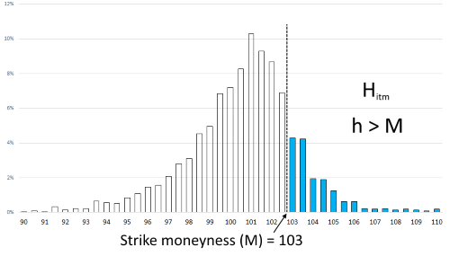
Here we have 647 such theoretical ITM expirations out of a total 4,277 days in our 17-year period. This is an estimation of the ITM expiration probability for the option with respective moneyness M of 103 and 2 weeks till expiration:
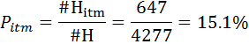
So, we have estimated, on the historical basis, that our call option would have expired ITM in 15.1% of all times in this 17-year period.
In the next step, for each of the 647 ITM returns, we can easily calculate a hypothetical value (payoff) of our call option at all these expiration moments. They are simply equal to the distance of the underlying price from the strike, or, in our terms, it is the difference between actual return (h) and option moneyness (M): EXPitm = h-M (for calls) and EXPitm =M-h (for puts).
To take an average of all these ITM payoffs, we use the following simple formula:
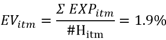
This is the desired estimation of the expected value of an option expired ITM. This value shows how far the underlying price has been overflying the 103 moneyness on average in history. It would have been a loss for an option seller and a profit for a buyer in all the cases of ITM expiration (disregarding initial option premium, of course).
Here we have the estimators of both crucial components of the Fair Value formula: the probability of expiration in-the-money and the expected value of the option in case of such an ITM expiration. And, finally, we can calculate the desired Fair Value of our call option just by multiplying these two values and discounting by e-rt to get the current value of the contract (in % of the underlying price):

As stated above, the fairness of this value means that both seller and buyer of an option have had zero total profit, should they have been making deals at this exact price in the past. Neither of them has had a statistical edge. In other words, if all trades with this options contract had been made at this price (0.29% of the underlying security price), both buyer and seller would have obtained a zero total profit at the end, not taking into account the transaction costs.
Note that the algorithm presented above is non-parametric, e.g., it does not assume any kind of distribution of security returns and does not need a model selection, calibration, or estimation of its parameters (mean, standard deviation, etc.). All we have done is just a simple calculation based on actual data of historical return for the selected time range.
Sequential vs. Daily returns (click to expand):
One important consideration is how to construct the initial set of historical return. There are two ways to do that:
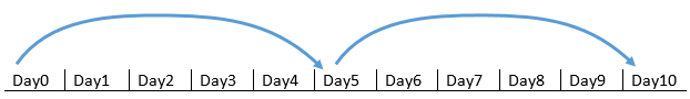
This method is close to real trading experience but has some serious drawbacks. First, it gives a rather small amount of returns to analyze, especially for longer intervals. For example, for a year we would have only 12 data points of monthly returns, which is not enough for building any reliable statistics. Second, we would inevitably “miss” many significant market moves up or down. For example, we would “jump over” market drawdowns or, vice versa, expire in the bottom of some rare trough.
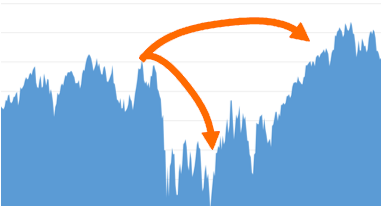
That might lead to the skewed assumption of outlier events by under- or overestimating their probabilities.
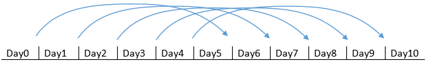
This approach does not look like a real-life experience because such daily “laddering” is rarely used in real trading. However, it gives much more statistical raw data than a sequential approach and does not omit significant market moves. That makes our probabilities estimation more robust and reliable.
For more, see the blog post Why OptionSmile is Better Than a Simple Backtesting.
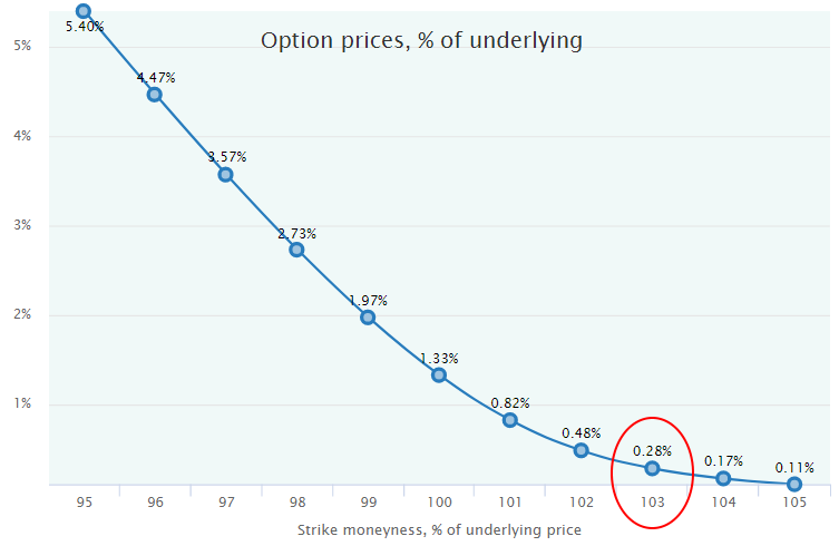
In the same way, we can apply this formula for each moneyness and time to expiration and come to the Fair Value of any option contract. Here are the call options Fair Values within the same expiration series but different moneyness. Our 103 call is circled.
In addition, we can reverse the Black-Scholes formula and calculate σ parameter implied by these option values and, hence, get the Fair Implied Volatility (IV) of each contract. Here is such a fair volatility smile (smirk, to be correct) for the call option prices calculated above.
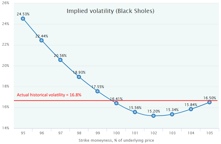
Note that the actual underlying price volatility — annualized standard deviation of returns — is 16.8%. Here we see a big discrepancy between this number and the Fair Implied Volatility calculated on the same dataset but more accurately, taking into account only particular strike and its ITM zone instead of overall average (standard) deviation from the mean.
Of course, the options market is familiar with that asymmetry (skewness) of returns distribution and adjusts the prices accordingly. That leads to the well-known volatility smile and time structure that constitute the whole volatility surface.
However, does it do that appropriately, comparing to the Fair Values? Our study shows that is not always the case; moreover, in most cases, market prices of opinions differ, and substantially, from their historically Fair Values. When it happens, one side of a trade (either buyer or seller) has a statistical edge over the opposite party.
Here is an example of such a situation with the same call options series where the actual Market Prices are overlapping the Fair Values of the same contacts.
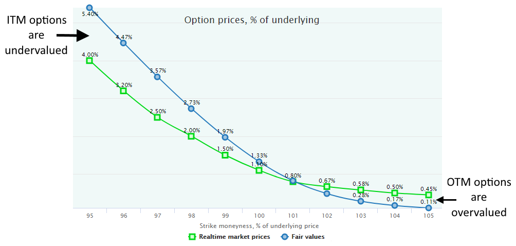
The position of these two lines means that ITM (moneyness <100) call options are undervalued by the market, and a buyer of such options has a theoretical statistical advantage. The opposite is true for the OTM part (moneyness>100), where the market is ready to pay for options more than their Fair Values. In such a market disposition, the obvious trading strategy should be to buy an ITM option and sell an OTM option (so-called debit call spread).
It should be already obvious that the difference between these two lines constitutes a mathematically expected profit/loss for a buyer/seller. The key term here is “expected” that is far from “guaranteed,” of course. This edge is only “statistical” in nature, and the profit calculated by the comparison of the Fair Value and market prices has not only the mean (expected value) but also the variance. That means that this profit will not be obtained in every trade, but will be realized as an average profit of some number of trades in future.
The OptionSmile methodology has some tools to deal with such a variance:
But, before diving into these topics, it is advisable to take a tour to another concept aimed at the solving of the problem with historical options market quotes, namely, their scarcity – see the article Historical Prices Estimation.
All the material presented in these methodological articles, but with more details, can be found in the book Option Fair Value: Finding a Statistical Edge in Options Trading. A free copy is available for registered users.
Read next: Historical Prices Estimation