All the material presented in these methodological articles, but with more details, can be found in the book Option Fair Value: Finding a Statistical Edge in Options Trading. A free copy is available for registered users.
The Fair Value of an option, being compared with current market price, provides the expected profit or loss for either buyer or seller.
Furthermore, it is also possible to apply this concept to find how this contract has been priced in history. This would be some kind of a “backtesting” that could reveal the areas of systematic market mispricing in the past. Also, read Why OptionSmile is Better Than Simple Backtesting.
The simplest approach is to take all the historical market quotes for similar contracts (the same moneyness and expiration), calculate an average price, and compare it with Fair Value to find a historical mispricing. Although that approach is quite reasonable, the problem here is the lack of historical data for options due to their expiration cycles. Actually, for an option, for each particular day, we have a new contract. Every day, it is getting closer to the expiration, and once it’s taken into the dataset for the average price calculation, it will not be suitable on the next day since it will have less time to expiration.
For the majority of underlying securities, there are usually just monthly options expiration cycles. For a few of the most popular stocks and ETFs, the weekly options series has been introduced only in recent years.
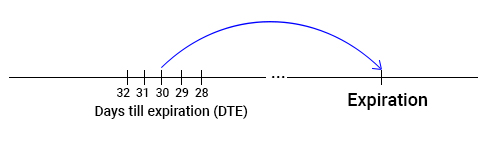
Let’s assume we are estimating the historical market mispricing of an option contract with 30 days-till-expiration (DTE). We have calculated its Fair Value and want to compare it with the average market price of such a contract in history. Having just 12 expiration dates per year, we get only 12 market quotes because this contract changes its DTE every day. One day it has 30 DTE, the next day – 29, then 28, and so on.
That amount of quotes is not enough for a reliable estimation of any statistics of a trading or hedging strategy. Add the fact that all these scarce quotes took place in different market regimes, and we get just a handful of data points and an extremely big variance of results. That would lead us to rather unreliable conclusions of market mispricing.
One workaround for this problem is to build a series of options theoretical quotes as if we have contracts expiring each day. The goal here is to answer the following question for each day in history: what would be the market price of an option contract today if it had any given (not exactly set by an options exchange) expiration date?
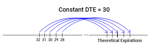
In this case, we would have not just 12 historical quotes per year but the set of prices for each trading day (around 252). That would give us a much wider statistical base and more reliable mispricing estimation. The only point missing in this logic is how to estimate these “pseudo-market” prices on each day in history with reasonable confidence.
Option Smile methodology exploits the Black-Scholes formula for this purpose. For all days in the given historical timeframe, we already have all the input parameters for this formula (underlying price, strike, interest rate, DTE) except for the balancing one—implied volatility. What if we could somehow “restore” this value for a given day and a given option contract?
To do this, we need some anchor, an indicator with strong correlation with the implied volatility of options. Of course, there are market indicators existing that capture the overall options market sentiment by measuring the expectations of future volatility implied by options prices. These indicators, known as Volatility Indices, are usually calculated and published by options exchanges. Perhaps, the most popular volatility index in the US market is VIX, created by the Chicago Board Options Exchange (CBOE) and representing the single measure of options prices on the S&P 500 Index with 30 calendar days to expiration on average. For more information, visit www.cboe.com/VIX
Because VIX has been calculated almost continuously, it is possible to get a history of such “snapshots” of the options market for a long period in the past with fine granularity. Then, having historical data of real market quotes of options on the S&P 500 Index on each day, we can build a model of the relationship between VIX and actual option prices expressed in their IVs for each moneyness/DTE. Finally, we can pair VIX data with options implied volatilities on each day when such quotes existed and build a regression model. It turns out that a simple linear regression is quite suitable for this purpose.
Linear regression (click to expand)
is a mathematical technique for modeling a relationship between two variables. One variable (y) is dependent on another, explanatory one (x). The model of linear regression has the following simple form:
y = a*x+b
Where a (slope) and b (intercept) are parameters of the model that must be calculated somehow, The simplest and most common method is the least-square estimation when we take some observed data of x and y and calibrate the model—find a and b so that all our data points have the least possible distance to the straight line that this model presents. By doing this, we find the “Best Fitting Line” for observed data points for x and y.
Finally, having the model, we can predict what value of y we would have given some value of x.
Having data pairs of VIX and actual IV of a contract for a set of historical dates, we can easily build such a model in the form of IV = a*VIX +b and estimate a and b based on our data.
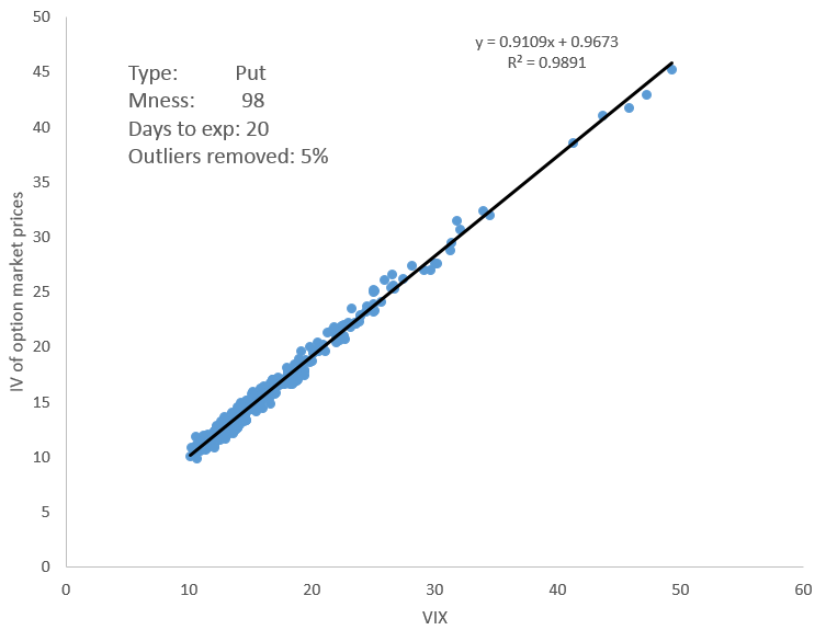
Here is a scatterplot with the relationship between VIX level and market implied volatilities of puts options on SPY with 98 moneyness and 10 trading DTE. The data source comprises the period 2005–2016, includes the IVs of the end-of-day option quotes (vertical axis), and the data set of end-of-day VIX values (horizontal axis).
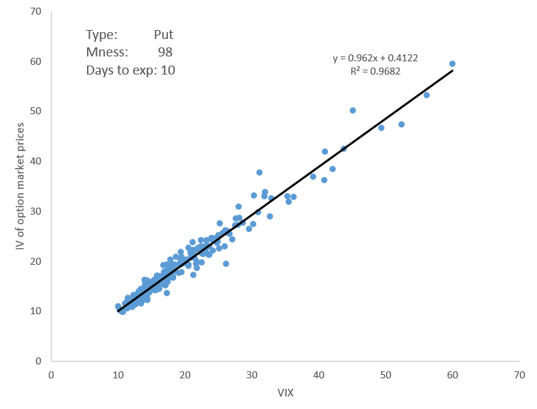
The very strong linear relationship between VIX and options IV is obvious from this chart. The coefficient of determination (R2) is also very high, around 0.97, meaning that about 97% of the variance of IV is explained by VIX.
No significant outliers are observed; but even if we had some, it would be possible to enhance the regression by excluding some small percentage of outliers from the sample. The following example with 20 trading DTE (4 weeks) and with the removal of 5% of outliers, demonstrates even stronger VIX-IV correlation and more quality regression.
Next, by taking the VIX value on any trading day in the past, we can estimate what IV of the contract with particular moneyness/DTE would be on this particular day—just by using the formula of linear regression and coefficients a and b calculated in advance. Finally, using this IV with the help of the Black-Scholes formula, we can “restore” the price of this option contract for any day, even though such a quote did not exist in reality.
Let’s take our first example with put option of 98 moneyness and DTE of 10. If, for instance, we had VIX of 15 at some moment in the past, we can assume that implied volatility of our contract would have been
IV = 0.962 * 15 + 0.4122 = 14.84
After that, with the help of the Black-Scholes formula (we already know all other inputs to it), we can find the option price corresponding to that 14.84% IV (it is 0.41% of the underlying price). We will call that value the Estimated Market Price, in contrast to the real actual market quote. That is actually an expected options price given some particular level of VIX.
Finally, by comparing these prices of options with their Fair Values, we can estimate what contracts (moneyness/DTE) have usually been under- or overvalued by the market on average in the past.
Even though these quotes did not exist in reality, the strong correlation between options IVs and VIX gives enough confidence in statistics derived from this data. After all, we are not interested in Estimated Market Prices on each particular day in the past. The focus of analysis is on the relationship between average prices and the Fair Values of the same contract. That gives us an ability to discover some market mispricing patterns in the historical data range.
In the same manner, we can actually recreate the whole “volatility surface” for each moment in history when VIX was calculated. Moreover, we get enough data points to ensure ourselves in this “average” historical market price.
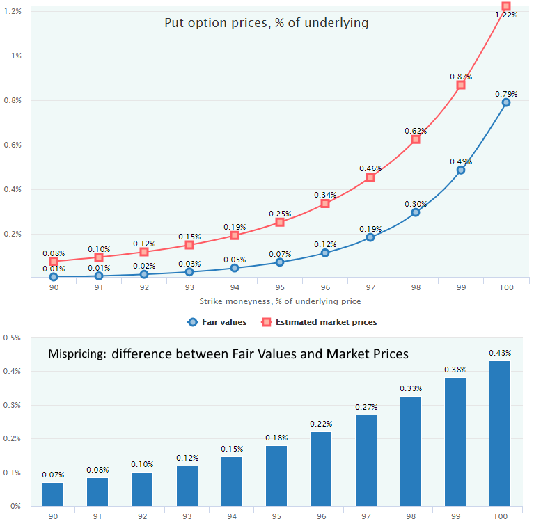
Here are the charts of the Estimated Market Prices with a comparison to the Fair Values of the SPY options from the example above. All calculations are made for the period 2010–2016 for OTM put options on SPY with trading DTE 10.
Here are the respective Black-Scholes implied volatilities (volatility smiles), for both Market Estimated Prices and Fair Values.
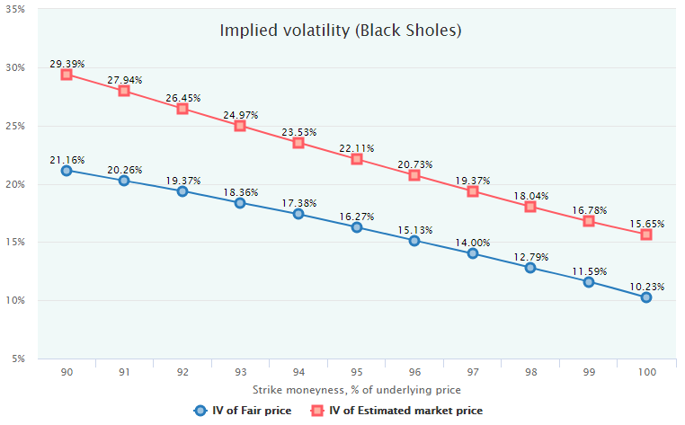
From these charts, the conclusion is evident: during the period of 2010–2016, put options with DTE 10 were systematically overpriced by the market. On average, selling puts would be a profitable strategy, and the exact average profit can be estimated by comparing the market prices of options with their respective Fair Values.
We also can calculate the expected profit/loss (PL) in another, more intuitive way. Obviously, we not only have the estimated market prices on each day in history, but we also have a privilege to know how exactly all these contracts had expired in the past and what exact payoff they had produced. Therefore, for each option quote in history, we already know the result of either buying or selling it. By the averaging of those PL values, we get an expected profit/loss for our option contract.
Having such a time series of profit/losses of buying or selling an option, we can go further and build the whole probability distribution of these PLs. That gives us an estimation of such indicators as standard deviation, tail risk, Sharpe ratio, and so forth. All these metrics can be calculated not just for a simple strategy of buying or selling of a single option contract, but for the whole set of option combinations. For more, see the article Fair Value of Option Strategies.
In all other methodology articles, we will overlay these Estimated Market Prices (red lines) against the Fair Values (blue lines) on charts to discover the historical mispricing of options. In practice, for the real trading, the real-time market prices should be used to estimate the expected profit/loss of a trade.
Read next: Market Regimes Filtering