One of the interesting questions regarding the Fair Value calculation approach is how the put-call parity is sustained for these values. Remember that this rule stands for the equivalence of difference between put and call prices on the same strike and difference between the strike and underlying price. If it is not sustained, the arbitrage opportunity arises.
For example, buying a put and selling a call on the same, strictly at-the-money strike equals the short position in the underlying security. If a put-call parity did not hold, it would be possible to hedge this position by buying an underlying security and get some return without any risk. In a risk-neutral paradigm, on which the Black-Scholes model is based, with such a combination we must always earn a return equal to the risk-free interest rate.
The exact formula for put-call parity is the following:
P – C = X*e-rt – S
P and С — prices of put and call options on the same strike (X), respectively
Х and S — strike and price of underlying
e-rt— discount factor with the risk-free continuous rate
For our purpose, we will use another form of this formula:
P – C = X – S*ert
That is, instead of discounting the strike (X), we take the future (expected) price of underlying at expiration date (S*ert). That value is often called a forward price of underlying.
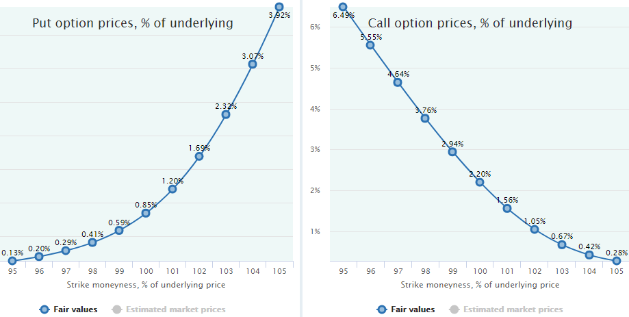
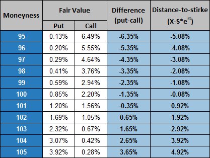
As an example, we take 20-day options on SPY and estimate their Fair Values for the 8.5-year period of March 2009 to September 2017 (it is just a voluntary choice since with all other periods, underlyings, and DTEs we will come to the same conclusions). For this period, the mean return of SPY has been 1.36% for the 20-day interval (including dividends). Let’s remember that number, it is important.
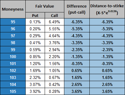
Here are the Fair Values of these puts and calls for moneyness from 95 to 105 (both ITM and OTM options):
Let’s take some annual risk-free rate, say 2%, and calculate the put-call parity for these options series:
As we can see from this data, the desired parity is far from being sustained. The difference between puts and calls (fourth column) is not equal to the difference between strike and forward price (fifth column) by far. Does it mean the whole model is wrong since it does not comply with the non-arbitrage requirement?
No, not at all. The model is correct. The reason for this discrepancy is that until now we have been thinking in a risk-neutral paradigm implying that investors are not risk-averse and all investment must earn a return equal to the risk-free interest rate. Hence, our underlying security must also have expected return equal to the risk-free rate. That is why we used this rate to calculate the forward price of underlying, namely, we multiplied S by the ert factor where r equals risk-free rate.
Of course, this assumption of the risk-neutrality is not supported by the real world. Investors in risky assets must earn a risk premium above the risk-free rate as a compensation for taking the additional risk. Otherwise, no one would invest in any assets other than risk-free bonds. Empirical data supports this and, of course, investors in equity indices like S&P 500 have historically been rewarded with a return above this rate by getting some equity premium.
If we now look more closely at the table above, namely at the difference between puts and calls (Column 4), we will see the suspicious consistency of its decimal part (.35 for negative difference and .65 for positive one). If we now deduct from this difference a distance from strike to underlying price (current, not forward) we will come to one number—1.35% on all strikes. This rate is suspiciously equal to the actual average rate of return of SPY for our sample, see above.
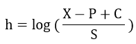
Of course, it is not by accident and it explains the strange noncompliance with the put-call parity rule. Let’s now calculate the forward price (S*ert) not with the risk-free rate but with the rate of actual return of SPY. Instead of rt = 2%*(20/252) = 0.16%—the risk-free rate for 20 working days—we take an actual return of 1.36% for this interval (to be more correct, we take a logarithm of it to get a continuous rate: r = ln(1.36%) = 1.35%).
Here we have come to the so-called real-world (empirical) put-call parity:
As we see from the fourth and fifth columns, parity is well-sustained in all strikes.
The conclusion here is obvious: as a discount rate, it is necessary to use the actual mean value of the underlying returns distribution on which Fair Values of options have been calculated, but not the risk-free rate. In other words, we must use the same probability measure as we applied in the calculation of option values, not risk-neutral measure. Only under this condition is the put-call parity with Fair Values held.
So, the generalized formula of put-call parity is as follows:
P – C = X – S*eh
h – expected rate of return of the underlying security
It is also possible to find a rate of underlying return implied by the option prices by solving this equation with respect to h:
Having actual market prices as P and C, this value (h) will be always close to the risk-free rate (minus dividends to get the total “cost of carry”) due to the ability of the risk-free arbitrage with these prices and the underlying security.